In this year’s ICML, some interesting work was presented on Neural Processes. See the paper conditional Neural Processes and the follow-up work by the same authors on Neural Processes which was presented in the workshop.
Neural Processes (NPs) caught my attention as they essentially are a neural network (NN) based probabilistic model which can represent a distribution over stochastic processes. So NPs combine elements from two worlds:
- Deep Learning – neural networks are flexible non-linear functions which are straightforward to train
- Gaussian Processes – GPs offer a probabilistic framework for learning a distribution over a wide class of non-linear functions
Both have their advantages and drawbacks. In the limited data regime, GPs are preferable due to their probabilistic nature and ability to capture uncertainty. This differs from (non-Bayesian) neural networks which represent a single function rather than a distribution over functions. However the latter might be preferable in the presence of large amounts of data as training NNs is computationally much more scalable than inference for GPs. Neural Processes aim to combine the best of these two worlds.
I found the idea behind NPs interesting, but I felt I was lacking intuition and a deeper understanding how NPs behave as a prior over functions. I believe, often the best way towards understanding something is implementing it, empirically trying it out on simple problems, and finally explaining this to someone else. So here is my attempt at reviewing and discussing NPs.
Before reading my post, I recommend the reader to take a look at both original papers. Even though here I discuss [NPs], you might find it easier to start with [conditional NPs] which are essentially a non-probabilistic version of NPs.
What is a Neural Process?
The NP is a neural network based approach to represent a distribution over functions. The broad idea behind how the NP model is set up and how it is trained is illustrated in this schema:

Given a set of observations $(x_i, y_i)$, they are split into two sets: “context points” and “target points”. Given the pairs $(x_c, y_c)$ for $c = 1, …, C$ in the context set and given unseen inputs $x_t^{\ast}$ for $t = 1, …, T$ in the target set, our goal is to predict the corresponding function values $y_t^{\ast}$. We can think of NPs as if they were modelling the target set conditional on the context. Information flows from the context set (on the left) to making new predictions on the target set (on the right) via the latent space $z$. The latter is essentially a finite-dimensional embedding of mappings from x to y. The fact that $z$ is a random variable makes NP a probabilistic model and lets us capture uncertainty over functions. Once we have trained the model, we can use our (approximate) posterior distribution of $z$ as a prior to make predictions at test time.
At first sight, the split into context and target sets may look like the standard train and test split of the data, but this is not the case, as the target set is directly used in training the NP model – our (probabilistic) loss function is explicitly defined over the target set. This will allow the model to avoid overfitting and achieve better out-of-sample generalisation. In practice, we would repeatedly split our training data into randomly chosen context and target sets to obtain good generalisation.
Let us consider two scenarios:
- Inferring a distribution over functions, based on a single data set
- Inferring a distribution over functions, when we have access to multiple data sets which we believe to be related in some way
The first scenario corresponds to a standard (probabilistic) supervised learning setup: Given a data set of $N$ samples, i.e. given $(x_i, y_i)$ for $i = 1, … ,N$, and assuming there is an underlying true $f$ which has generated the $y_i = f(x_i)$ values, our goal is to learn the posterior distribution over $f$ and use it to get predictive densities at test points $f(x^{\ast})$.
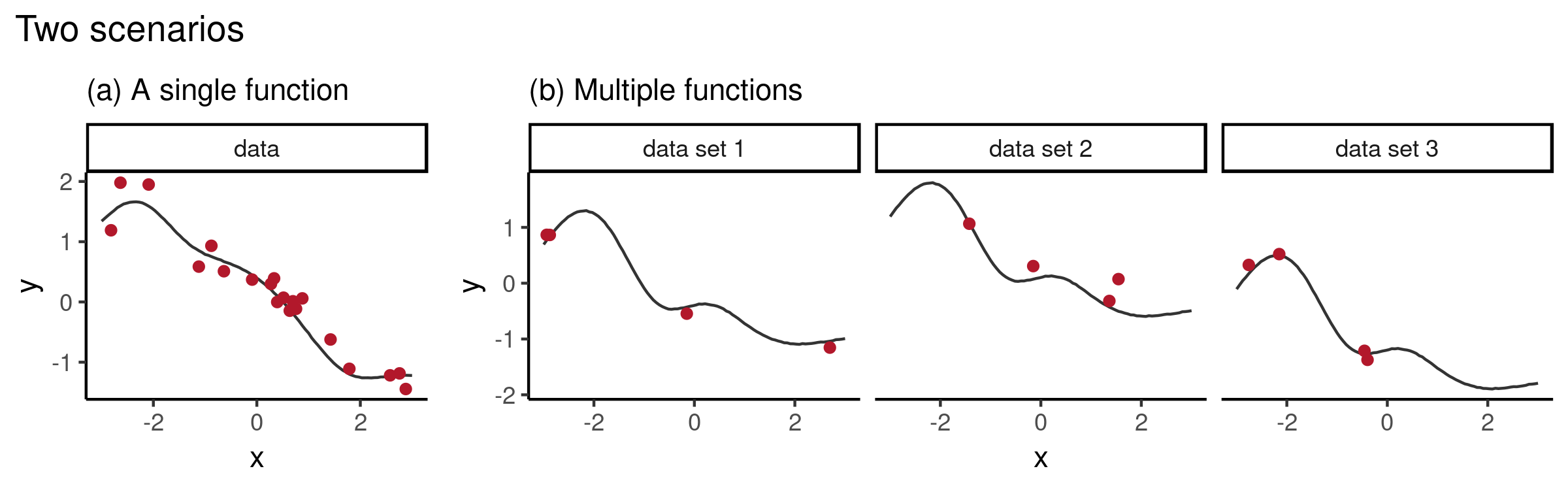
The second scenario can be seen from the meta-learning viewpoint. Given $D$ data sets $d = 1, …, D$, each consisting of $N_d$ pairs $(x_i^{(d)}, y_i^{(d)})$, if we assume that every data set $d = 1, …, D$ has its own underlying function $f_d$ which has generated the values $y_i = f_d(x_i)$, we might want to learn the posterior of every $f_d$ as well as generalise to a new data set $d^{\ast}$. The latter is especially useful when every data set has only a small number of observations. This information sharing is achieved by specifying that there exists a shared process which underlies all functions $f_d$. For example, in the context of GPs, one can assume that $f_d \sim \mathcal{GP}$ share kernel hyperparameters. Having learned the shared process, when given a new data set $d^{\ast}$, one can use the posterior over functions as a prior and carry out few-shot function regression.
The reason I wanted to highlight these two scenarios is the following. Usually, in the most standard setting, GP-regression is carried out under the first scenario. This tends to work well even when $N$ is small. However, the motivation behind NPs seems to be mainly coming from the meta-learning setup – in this setting the latent $z$ can be thought of as a mechanism to share information across different data sets. Nevertheless, having elements of a probabilistic model, NPs should be applicable in both scenarios. Below we will investigate how NPs behave when trained only on a single data set, as well as the second setup where we have access to a large number of function draws in order to train the NP.
How are NPs implemented?
Here is a more detailed schema of the NP generative model:

Going through this generative mechanism step-by-step:
- First, the context points $(x_c, y_c)$ are mapped through a NN $h$ to obtain a latent representation $r_c$.
- Then, the vectors $r_c$ are aggregated (in practice: averaged) to obtain a single value $r$ (which has the same dimensionality as every $r_c$).
- This $r$ is used to parametrise the distribution of $z$, i.e. $p(z | x_{1:C}, y_{1:C}) = \mathcal{N}(\mu_z( r ), \sigma_z^2( r ))$
- Finally, to obtain a prediction at a target $x_t^{\ast}$, we sample $z$ and concatenate this with $x_t^{\ast}$, and map $(z, x_t^{\ast})$ through a NN $g$ to obtain a sample from the predictive distribution of $y_t^{\ast}$.
Inference for the NP is carried out in the variational inference framework. Specifically, we introduce two approximate distributions:
- $q(z | \text {context})$ to approximate the conditional prior $p(z | \text {context})$
- $q(z | \text {context}, \text {target})$ to approximate the respective $p(z | \text {context}, \text {target})$ where we have denoted $\text {context} := (x_{1:C}, y_{1:C})$ and $\text {target} := (x_{1:T}^{\ast}, y_{1:T}^{\ast})$.
The approximate posterior $q(z | \cdot)$ is chosen to have the specific form as illustrated in the inference model diagram below. That is, we use the same $h$ to map both the context set as well as the target set to obtain the aggregated $r$, which in turn is mapped to $\mu_z$ and $\sigma_z$. These parametrise the approximate posterior $q(z | \cdot) = \mathcal{N}(\mu_z, \sigma_z)$.

The variational lower bound
$$\text {ELBO} = \mathbb{E}_{q(z | \text {context}, \text {target})} \left[ \sum_{t=1}^T \log p(y_t^{\ast} | z, x_t^{\ast}) + \log \frac{q(z | \text {context})}{q(z | \text {context}, \text {target})} \right]$$
contains two terms. The first is the expected log-likelihood over the target set. This is evaluated by first sampling $z \sim q(z | \text {context}, \text {target})$, as indicated on the left part of the inference diagram, and then using these $z$ values for predictions on the target set, as on the right part of the diagram. The second term in ELBO has a regularising effect – it is the negative KL divergence between $q(z | \text {context}, \text {target})$ and $q(z | \text {context})$. Note that this differs slightly from the most commonly encountered variational inference setup with $\text{KL}(q || p)$, where $p$ would be the prior $p(z)$. This is because in our generative model, we have specified a conditional prior $p(z | \text {context})$ instead of directly specifying $p(z)$. As this conditional prior depends on $h$, we do not have access to its exact value and instead need to use an approximate $q(z | \text {context})$.
Experiments
NP as a prior over functions
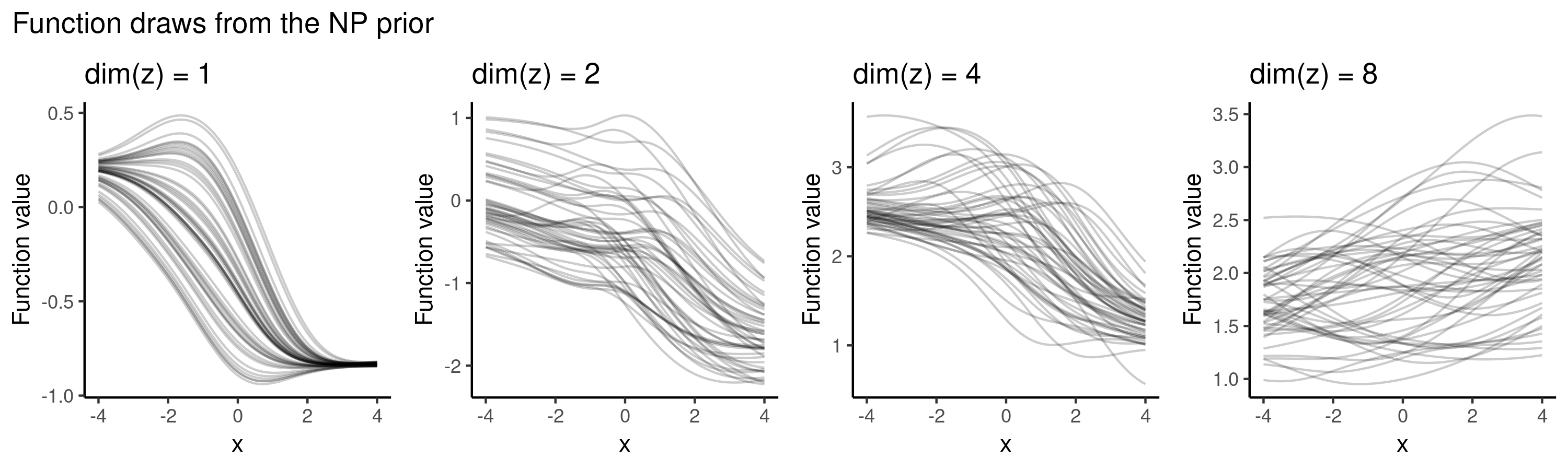
Let’s start by exploring the behaviour of NPs as a prior over functions, i.e. in the setting where we haven’t observed any data and haven’t yet trained the model. Having initialised the weights (here I initialised them independently from a standard normal), we can sample $z \sim \mathcal{N}(0, I)$ and generate from the prior predictive distribution over a grid of $x^{\ast}$ values to plot the functions.
As opposed to GPs which have interpretable kernel hyperparameters, the NP prior is much less explicit. There are various architectural choices involved (such as how many hidden layers to use, what activation functions to use etc) which all implicitly affect our prior distribution over the function space.
For example, when using sigmoid activations and varying the dimensionality of $z$ in $\{1, 2, 4, 8\}$, typical draws from the (randomly initialised) NP prior may look as follows:
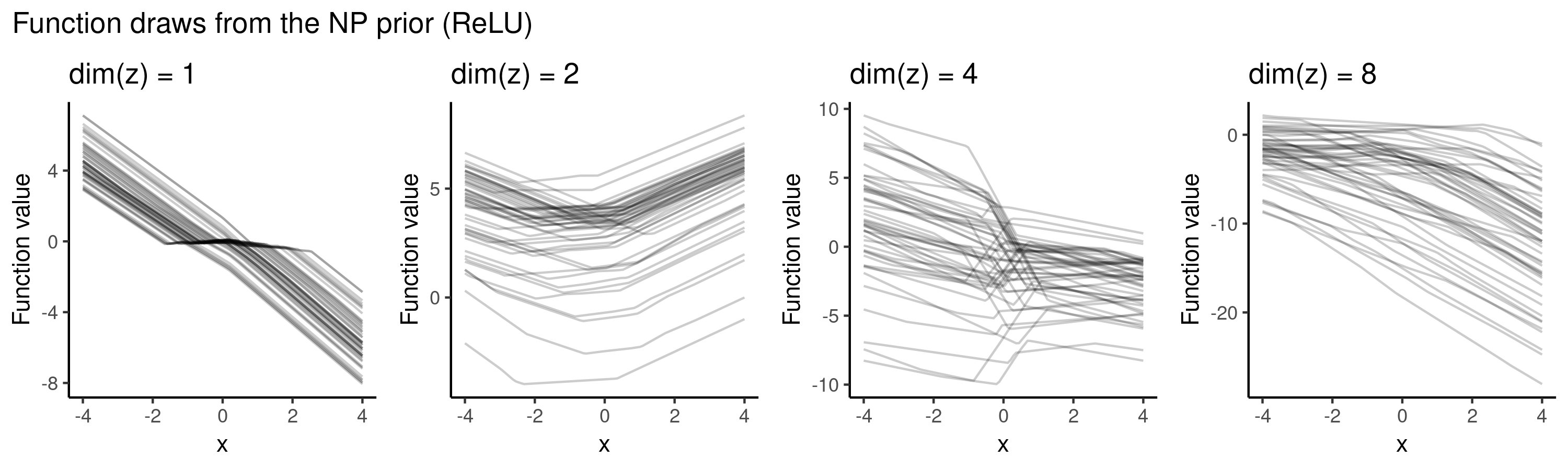
But when deciding to use the ReLU activations instead, we have placed the prior probability mass over a different set of functions:
Training NP on a small data set
Suppose all we have is the following five data points:

The training procedure for NPs will involve separating the context set and target set. One option is to use a fixed size context set, another is to cover a wider range of scenarios by training using varying context set sizes (e.g. at every iteration we could randomly draw the number of context points from the set $\{1, 2, 3, 4\}$). Once we have trained the model on these random subsets, we use the trained model as our prior and now condition on all of our data (i.e. we take all these five points to be the context points) and plot draws from the posterior. The animation below illustrates how the predictive distribution of the NP changes as it is being trained:
So the NP seems to have successfully learned a distribution over mappings which go through all of our five points. Now let’s explore how well it generalises to other mappings, i.e. what happens if we use this trained NP for prediction on a different context set. Here is the posterior when conditioning on the red points instead:
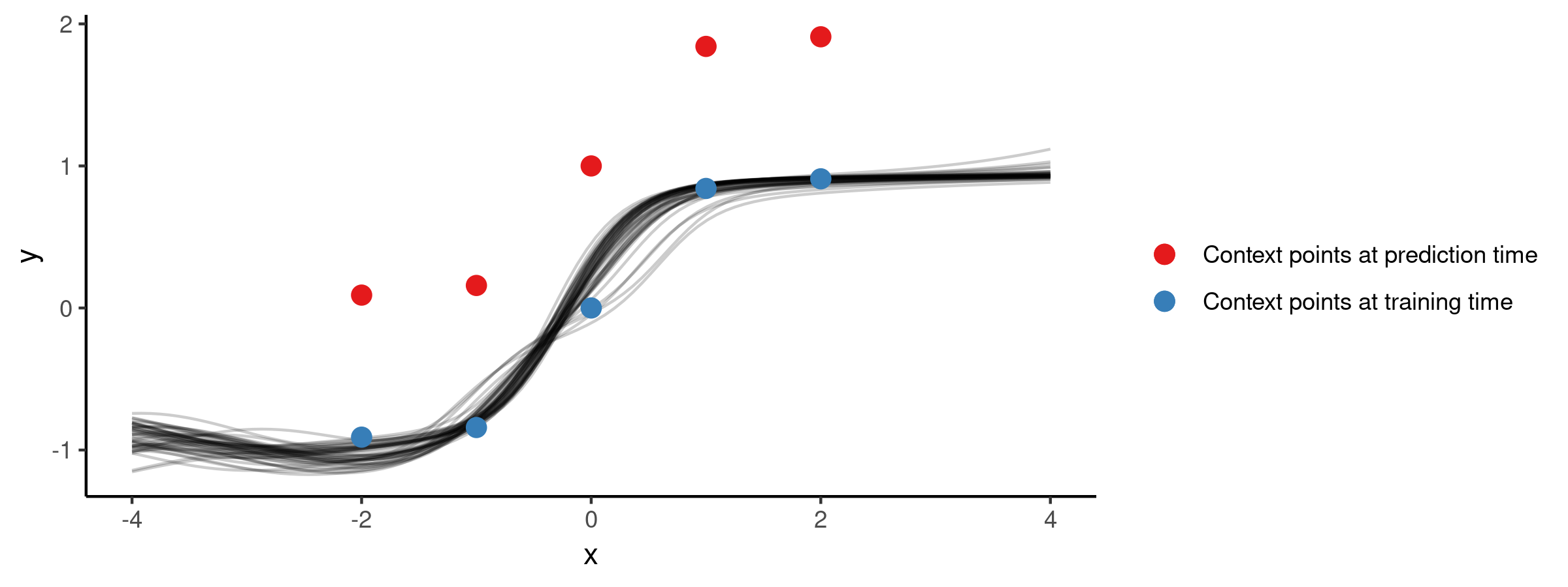
Not very surprisingly, the flexible NP model which was trained only on subsets of the five blue points, doesn’t generalise to a different set of context points. To get a model which would generalise better, we could consider (pre)training the NP on a larger set of functions.
Training NPs on a small class of functions
So far, we have explored the training scenario using a single (fixed) data set. To have an NP which would generalise similarly to GPs, it seems that we should train it on a much larger class of functions. But before that, let’s explore how NPs behave in a simpler setting.
That is, let’s consider a toy scenario, where instead of a single function we observe a small class of functions. Specifically, let’s consider all functions of the form $a \cdot \sin(x)$ where $a \in [-1, 1]$.
It would be interesting to see:
- Is the NP able to capture this class of functions
- Will it generalise beyond this class of functions
Let’s use the following training procedure:
- Draw $a$ uniformly $a \sim U(-2, 2)$
- Draw $x_i \sim U(-3, 3)$
- Define $y_i := f(x_i)$, where $f(x) = a \sin(x)$
- Divide pairs $(x_i, y_i)$ randomly into context and target sets and perform an optimisation step
- Repeat
Here we used a two-dimensional $z$ so that we could visualise what the model has learned. Having trained the NP, we visualised the function draws corresponding to various $(z_1, z_2)$ values on a grid, as shown below:
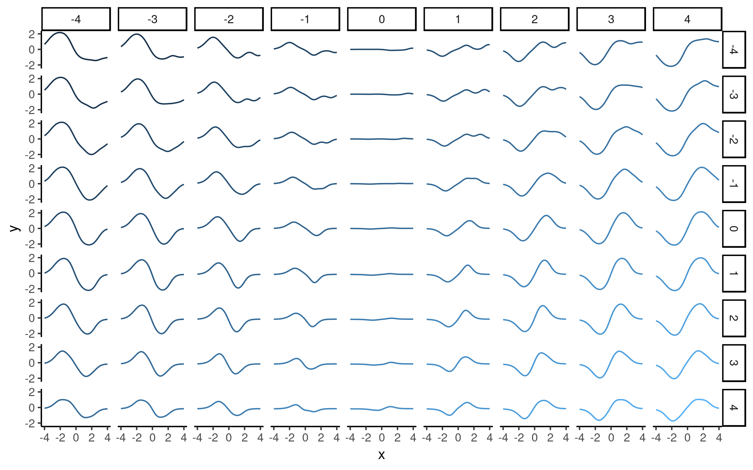
It seems that the direction from left-to-right essentially encodes our parameter $a$. Here is another visualisation of the same effect, where we vary one of the latent dimensions (either $z_1$ or $z_2$):
Note that above we did not use any context set at prediction time, but simply pre-specified various $(z_1, z_2)$ values. Now let’s look into using this trained model for predicting.
Taking the context set to be the point $(0, 0)$, shown on the left, will result in quite a broad posterior which looks quite nice, covering functions which resemble $a \sin(x)$ for a certain range of values of $a$ (but note that not for all $a \in [-2, 2]$ it was trained on).
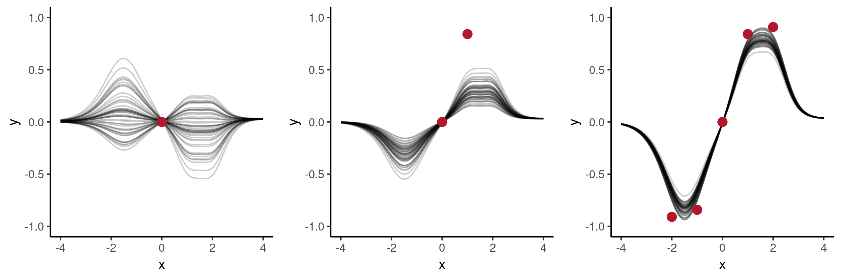
Adding a second context point $(1, \sin(1))$ will result in the posterior shown in the middle. The posterior has changed compared to the previous plot, e.g. functions with a negative values of $a$ are not included any more, but none of the functions goes through the given point. When increasing the number of context points which follow $f(x) = 1.0 \sin(x)$ then the NP posterior will become reasonably close to the true underlying function, as shown on the right.
Now let’s explore how well the trained NP will generalise beyond the class of functions it was trained on. Specifically, let’s explore how it will generalise to the following functions $2.5 \sin(x)$ and $| \sin(x) |$. The first requires some extrapolation from the training data. The second one has a similar shape to the functions in training set but unlike the rest its values are non-negative.
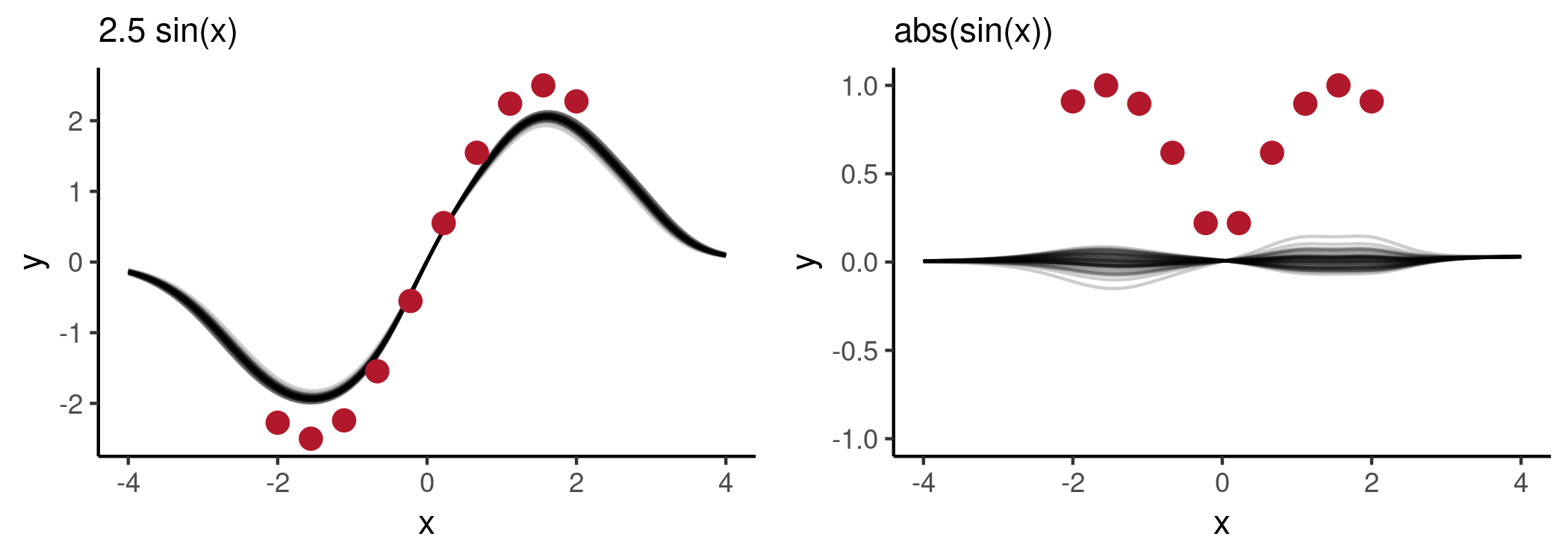
As seen from the plots, the NP has not been able to generalise beyond what it had seen during training. In both cases, the model behaviour is somewhat expected (e.g. on the left, $a=2$ corresponds to the best fit within the class of functions the model has seen). However, note that there is not much uncertainty in the NP predictive distributions. Of course over-confident predictions are not specific to NPs, however their black-box nature may make them more difficult to diagnose, compared to more interpretable models.
Training NPs on functions drawn from GPs
Based on experiments so far, it seems that NPs are not out-of-the-box replacements for GPs, as the latter have more desirable properties regarding posterior uncertainty. In order to achieve a similar behaviour with an NP, we could train it using a large number of draws from a GP prior. We could do it as follows:
- Draw $f \sim \mathcal{GP}(0, k_{\theta}(\cdot))$
- Draw $x_i \sim U(-3, 3)$
- Define $y_i := f(x_i)$
- Divide pairs $(x_i, y_i)$ randomly into context and target sets and perform an optimisation step
- Repeat
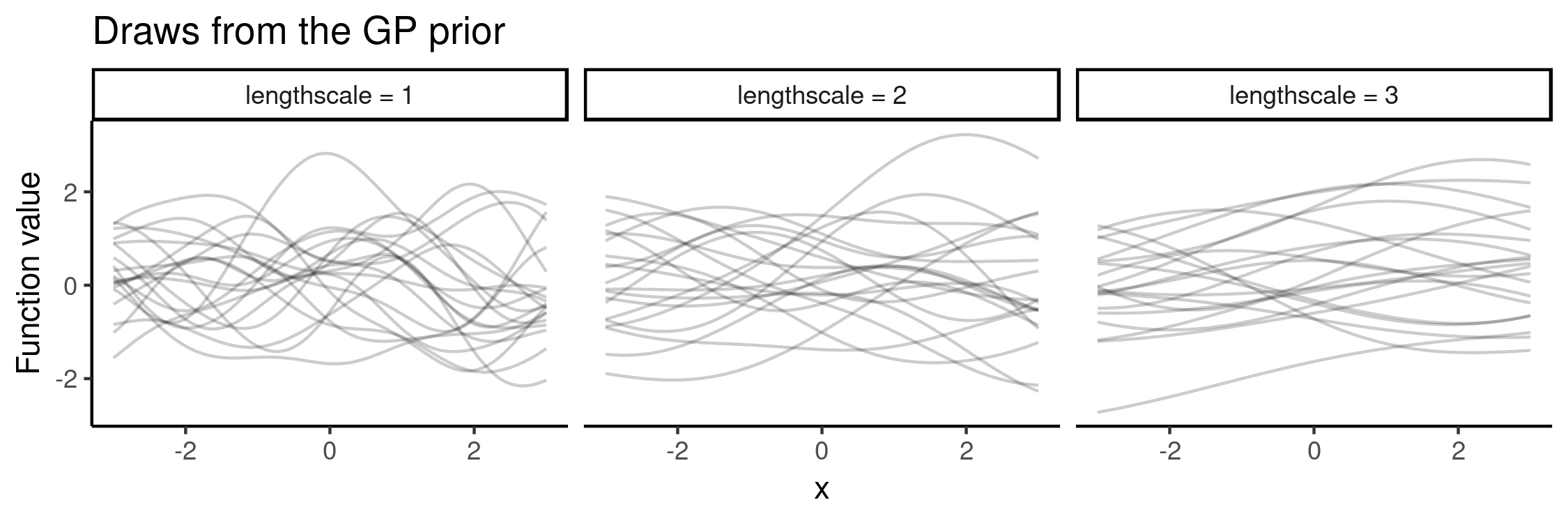
The above procedure can be carried out with fixed kernel hyperparameters $\theta$ or a mixture of different values. The RBF (or squared exponential) kernel has two parameters: one controls the variance (essentially the range of function values) and the other “wigglyness”. The latter is called the lengthscale parameter and its effect is illustrated here, by drawing functions from the GP prior with lengthscale values in $\{1, 2, 3\}$:
To cover a variety of functions in the NP training, we could specify a prior $p(\theta)$ where to draw samples from. In this toy experiment, I varied lengthscale, as above, uniformly in $\{1, 2, 3\}$. As previously, choosing the latent $z$-space to be 2D, we can visualise what the NP has learned:
This looks pretty cool! The NP has learned the two-dimensional $z$ space where we can smoothly interpolate between different functions.
Now let’s explore the predictions we get using this NP, and let’s see how its behaviour compares to a Gaussian Process posterior. Using an increasing number of context points $\{3, 5, 11\}$, let’s consider two functions:
First, using a relatively smooth function $f(x) = \sin(0.5x)$, the predictions look as follows:
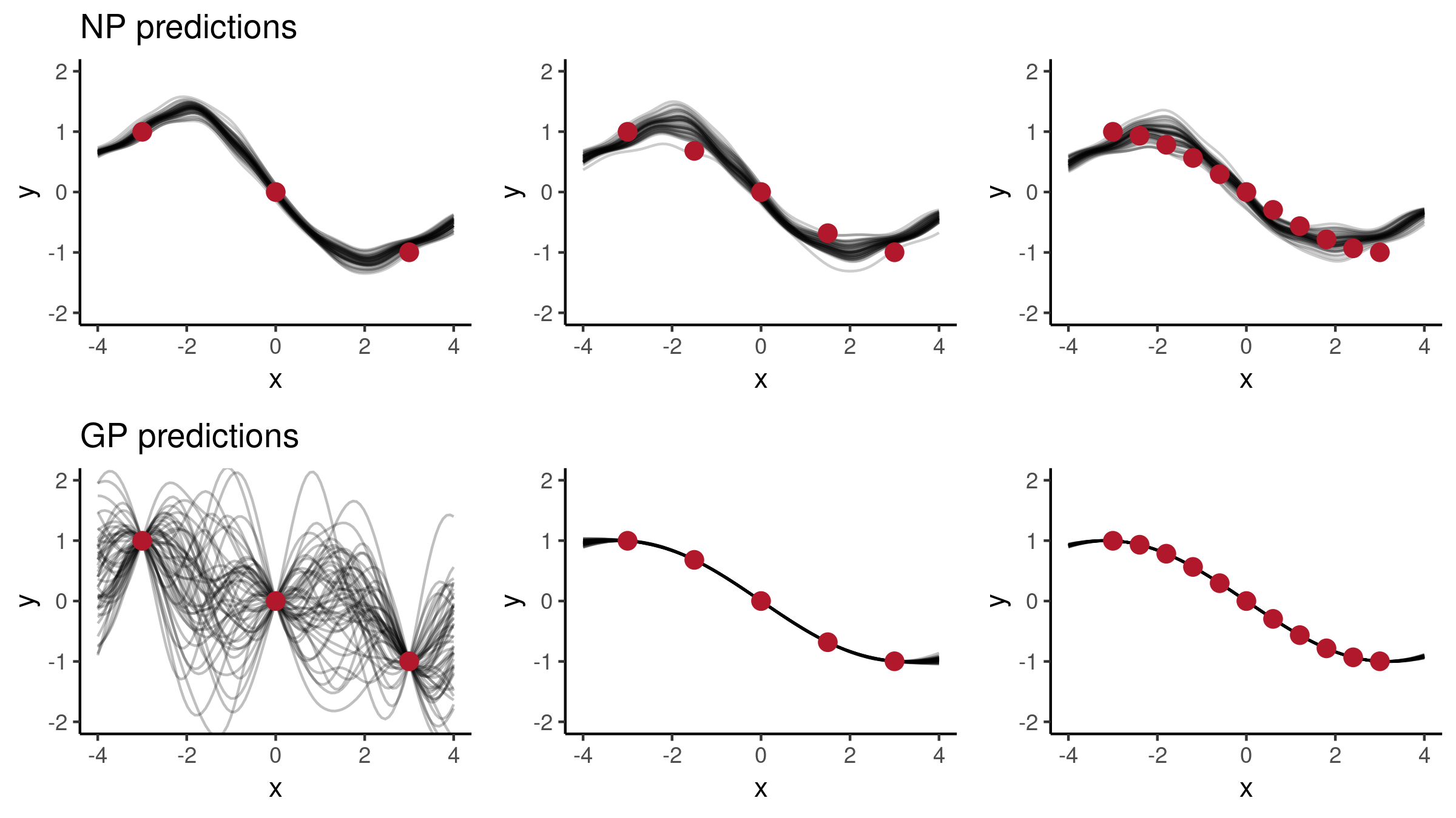
Second, let’s consider $f(x) = \sin(1.5x)$:
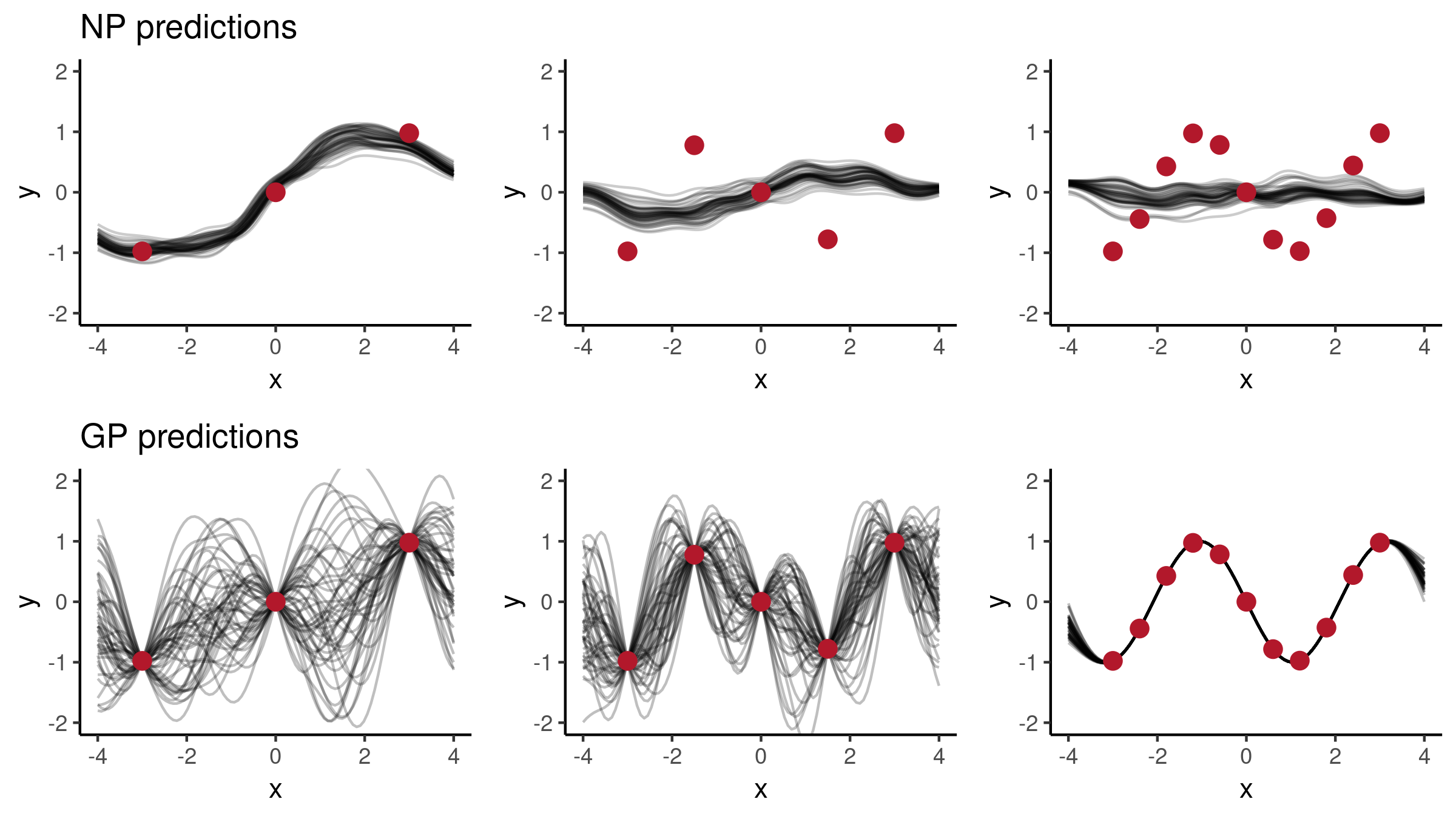
In the first case, the NP predictions follow the observations quite closely, whereas in the second case, with three observations it looks good, but when given more points it hasn’t been able to capture the pattern. This effect is quite likely due to our architectural choices to use quite small NNs and a low-dimensional $z$. In order to improve the model behaviour so that it would resemble GPs more closely, we could consider applying the following changes:
- Using only a 2D $z$-space might be quite restrictive in what we are able to learn, we could consider using a higher-dimensional $z$. And similarly for $r$.
- We could consider using a larger number of hidden units in NNs $h$ and $g$, and consider making them deep.
- Observing a larger number of function draws as well as a larger variety of functions (i.e. more variability in GP kernel hyperparameters) during the training phase could lead to better generalisation.
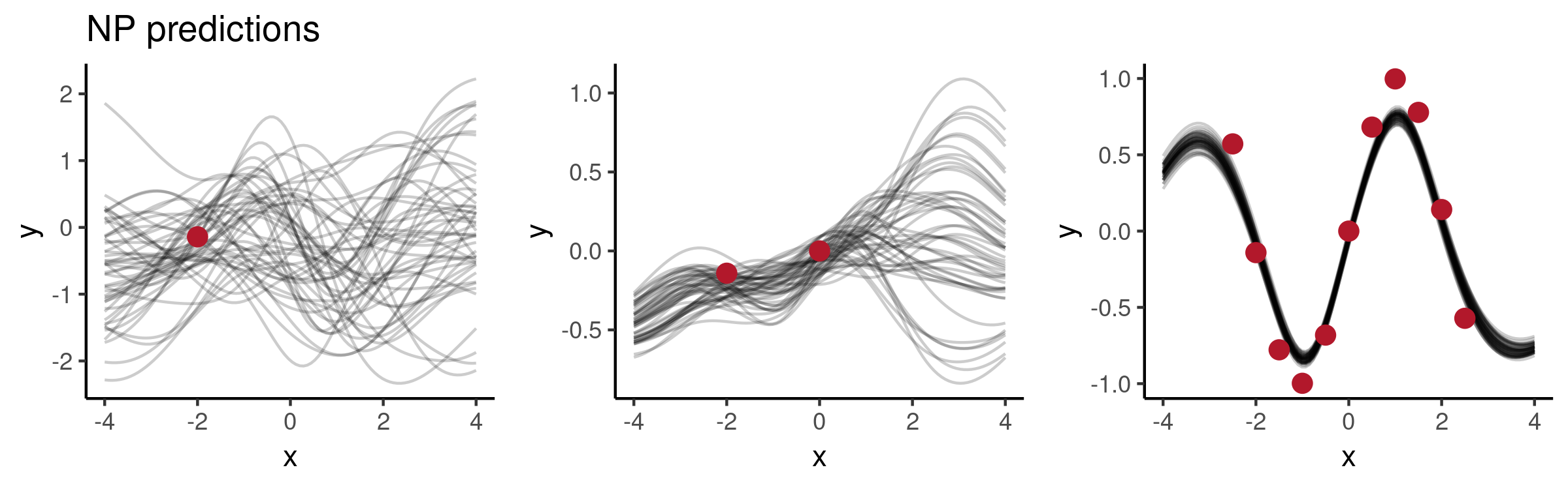
Such changes can indeed lead to more desirable results. For example, having increased $\text {dim}( r )$ to 32 and $\text {dim}(z)$ to 4 together with a larger number of hidden units in $h$ and $g$, we observe much nicer behaviour:
Conclusions
Even though Neural Processes combine elements from both NNs and GP-like Bayesian models to capture distributions over functions, on this spectrum NPs lie closer to neural models. By making careful choices regarding the neural architectures as well as the training procedure for NPs, it is possible to achieve desirable model behaviour, e.g. GP-like predictive uncertainties. However, these effects are mostly implicit which make NPs more challenging to interpret as a prior.
Implementation
My implementation using TensorFlow in R (together with code for the experiments above) is available in github.com/kasparmartens/NeuralProcesses.
Acknowledgements
I would like to thank Hyunjik Kim for clarifying my understanding of the NP papers, Jin Xu for sharing his results on NPs (which stimulated me to think about more complex NNs), Tanel Pärnamaa and Leon Law for their comments, and Chris Yau for being an awesome supervisor.